
Introduction
In earlier posts, I opined that the behaviour of various climate subsystems showed greater complexity in the Late Pleistocene than in the early Pleistocene. This opinion is shaped by observations of the behaviour of these varying subsystems (Himalayan monsoon strength, global ice volume, and oceanographic conditions) inferred from proxy records up to about 2 million years in length.
Any such argument would be strengthened by a number. So the challenge I will address over the next few posts in this series will be--how to characterize the complexity of the output of a dynamic series by a single number. After all, in order to compare complexity between two periods, it would be helpful to have a single parameter to compare.
The principal information theoretic concept we shall use is Shannon's (1949) measurement of entropy. The trick is deciding how to apply this parameter.
Entropy of the epsilon machine for the ice volume proxy
Let's look at epsilon machine reconstructions of the ice volume proxy.

Three separate first-order epsilon machines describe portions of the Early Pleistocene variations in the ice volume proxy. A1 represents a minimum ice state, A2 is roughly what goes for an interglacial at present, and A3 is the maximum ice state of the early Pleistocene, which would pass for a minor glacial event in the late Pleistocene.

The Mid-Pleistocene epsilon machine looks more complex.

The Late Pleistocene epsilon machine reconstruction for the ice volume looks to be more complex than any of the Early Pleistocene reconstructions. But is it? How can we tell?
The approach we will try here is to characterize the complexity by the entropy of all of the state transitions. Entropy is expressed as -Σp(i)log p(i) for all values of p(i).* Entropy is considered to be a measure of the "information" in a stream of data. This expression is normally applied in systems where Σp(i) = 1, a condition not met in the figures above. The probabilities of each pathway leading from each of the predictive states adds up to 1; so that the total of all "probabilities" adds up to the number of predictive states in the epsilon machine (two or three in the Early Quaternary, four in the mid Quaternary, six in the late Quaternary.
Do we add up the probabilities as they appear? Should we divide all probabilities by the total number of predictive states so we end up with Σ p(i) = 1? Should we weight the various probabilities to reflect the relative importance of an individual predictive state?
Let's see what happens.
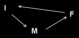
First off, consider a system based not on the proxy data, but on a model. Say, the Late Quaternary global ice volume model of Paillard (1998).

Quite provocative given the current state of the economy! Actually, the I stands for interglacial regime, the M for mild glacial regime, and the F for full glacial regime. The system bumps along from state to state, but there are no probabilities listed as there is only one possible successor state from each predictive state.
Is the above system more complex, less complex, or the same as one with a single state--say, "I".
From a dynamic system, which would use topological arguments--both systems would be equally complex (or simple, in this case), as there is no choice of successor state from each predictive state. From an information sense, it is not at all clear the two systems are the same.
I M F I M F I M F I M F I M F I M F . . .
I I I I I I I I I I I I I I I I I I I I I I . . .
It depends on whether you allow yourself to 'group' the Is, Ms, and Fs into words, which repeat. From a geological perspective, there is a difference in the complexity between the two systems--having three separate predictive states is different than having a single repeated predictive state.
However, if we calculate entropy [-Σp(i)log p(i)] for all the states in both systems, we come up with a value of zero. This is because the probability of each transition (I → M, M→ F, F → I or I → I in the second example) is 1. If, on the other hand, we establish the probability of each of the transitions (I → M, M → F, and F → I) as 1/3, then the entropy is 1.585, as compared to zero for the system with a single predictive state.
The implied complexity is 3x greater for the I M F system as compared to I. Seems reasonable. Now let's consider the epsilon machine construction for the Early Quaternary ice volume proxy.
There are two possibilities to recalculating the probabilities of each transition for α1, for instance: we could divide each of the probabilities by by the number of predictive states (remembering that the probability on the unlabelled A1 → A3 arrow is 1), or we could multiply the probability of each transition by the probability of the originating predictive state. In the interval from 1870-1700 ka, we find p(A1) = 0.2, p(A2) = 0.4, p(A3) = 0.4.
By method 1, the entropy for α1 is 2.13. By method 2, the entropy for α1 is 2.17. Not too different.
By both methods, the entropy for both α2 and α3 is 1.
For the Mid Pleistocene, the entropy for α4 (by method 1) is 3.23. We observe p(A1) = 0.19, p(A2) = 0.125, p(A3) = 0.31, p(A4) = 0.375, so by method 2, entropy for α4 is 3.21. Again, not much different from method 1.
For the Late Pleistocene, the entropy of α5 (by method 1) is 3.42. We observe p(A1) = 0.027, p(A2) = 0.243, p(A3) = 0.243, p(A4) = 0.297, p(A5) = 0.162, p(A6) = 0.027. The entropy of α5 is 2.85, which is considerably lower than by method 1. I think this is because observations of A1 and A6 are rare, as these predictive states are only observed once each during the Late Pleistocene.
Entropy of epsilon machines for paleomonsoon strength proxy
Now consider the reconstructed epsilon machines for the paleomonsoon strength proxy. We shall only use method 2 in calculating entropy.

Three predictive states in the Early Quaternary, dominated by M1 and M2. Given p(M1) = 0.50, p(M2) = 0.41, p(M3) = 0.09, then the entropy of μ1 is 1.83.

In the Late Quaternary, there are six predictive states, with observed probabilities as follows: p(M1) = 0.4, p(M2) = 0.2, p(M3) = 0.17, p(M4) = 0.1, p(M5) = 0.1, p(M6) = 0.03. The entropy of μ2 is 3.67.
Conclusions
Method 1 is the easier calculation, however method 2 is a better calculation. However, method 1 can be used as long as the distribution of predictive states is not too far from even.
In summary
Time Entropy (ice volume) Entropy (paleomonsoon)
Late Pleistocene 2.85 3.67
Mid-Pleistocene 3.21 1.83
Early Pleistocene 1-2.1 1.83
By this test, the behaviour of the climate system has been more complex in the Late Pleistocene than it was in the Early Pleistocene.
In our next installment, we look at how we can use the characterize the complexity for the probability density calculation for each window shown here, to give us a nice smooth graph of complexity of the climate system through time.
References
Crutchfield, J. P., 1994. The calculi of emergence: Computation, dynamics, and induction. Physica D 75: 11-54.
Gipp, M. R., 2001. Interpretation of climate dynamics from phase space portraits: Is the climate system strange or just different? Paleoceanography, 16, 335-351.
Kukla, G., Z. S. An, J. L. Melice, J. Gavin, and J. L. Xiao, 1990. Magnetic susceptibility record of Chinese loess. Trans. R. Soc. Edinburgh Earth Sci., 81: 263-288.
Paillard, D., 2001. Glacial cycles: Toward a new paradigm. Reviews of Geophysics, 3: 325-346.
Shackleton, N. J., A. Berger, and W. R. Peltier, 1990. An alternative astronomical calibration of the Lower Pleistocene timescale based on ODP site 677, Trans. R. Soc. Edinburgh, Earth Sci., 81: 251-261.
Shannon, Claude (1949). "Communication Theory of Secrecy Systems". Bell System Technical Journal 28 (4): 656–715.
* We calculate all logarithms in a base of 2, in accordance with the nerds who came up with this concept.
In earlier posts, I opined that the behaviour of various climate subsystems showed greater complexity in the Late Pleistocene than in the early Pleistocene. This opinion is shaped by observations of the behaviour of these varying subsystems (Himalayan monsoon strength, global ice volume, and oceanographic conditions) inferred from proxy records up to about 2 million years in length.
Any such argument would be strengthened by a number. So the challenge I will address over the next few posts in this series will be--how to characterize the complexity of the output of a dynamic series by a single number. After all, in order to compare complexity between two periods, it would be helpful to have a single parameter to compare.
The principal information theoretic concept we shall use is Shannon's (1949) measurement of entropy. The trick is deciding how to apply this parameter.
Entropy of the epsilon machine for the ice volume proxy
Let's look at epsilon machine reconstructions of the ice volume proxy.

Three separate first-order epsilon machines describe portions of the Early Pleistocene variations in the ice volume proxy. A1 represents a minimum ice state, A2 is roughly what goes for an interglacial at present, and A3 is the maximum ice state of the early Pleistocene, which would pass for a minor glacial event in the late Pleistocene.

The Mid-Pleistocene epsilon machine looks more complex.

The Late Pleistocene epsilon machine reconstruction for the ice volume looks to be more complex than any of the Early Pleistocene reconstructions. But is it? How can we tell?
The approach we will try here is to characterize the complexity by the entropy of all of the state transitions. Entropy is expressed as -Σp(i)log p(i) for all values of p(i).* Entropy is considered to be a measure of the "information" in a stream of data. This expression is normally applied in systems where Σp(i) = 1, a condition not met in the figures above. The probabilities of each pathway leading from each of the predictive states adds up to 1; so that the total of all "probabilities" adds up to the number of predictive states in the epsilon machine (two or three in the Early Quaternary, four in the mid Quaternary, six in the late Quaternary.
Do we add up the probabilities as they appear? Should we divide all probabilities by the total number of predictive states so we end up with Σ p(i) = 1? Should we weight the various probabilities to reflect the relative importance of an individual predictive state?
Let's see what happens.
First off, consider a system based not on the proxy data, but on a model. Say, the Late Quaternary global ice volume model of Paillard (1998).
Quite provocative given the current state of the economy! Actually, the I stands for interglacial regime, the M for mild glacial regime, and the F for full glacial regime. The system bumps along from state to state, but there are no probabilities listed as there is only one possible successor state from each predictive state.
Is the above system more complex, less complex, or the same as one with a single state--say, "I".
From a dynamic system, which would use topological arguments--both systems would be equally complex (or simple, in this case), as there is no choice of successor state from each predictive state. From an information sense, it is not at all clear the two systems are the same.
I M F I M F I M F I M F I M F I M F . . .
I I I I I I I I I I I I I I I I I I I I I I . . .
It depends on whether you allow yourself to 'group' the Is, Ms, and Fs into words, which repeat. From a geological perspective, there is a difference in the complexity between the two systems--having three separate predictive states is different than having a single repeated predictive state.
However, if we calculate entropy [-Σp(i)log p(i)] for all the states in both systems, we come up with a value of zero. This is because the probability of each transition (I → M, M→ F, F → I or I → I in the second example) is 1. If, on the other hand, we establish the probability of each of the transitions (I → M, M → F, and F → I) as 1/3, then the entropy is 1.585, as compared to zero for the system with a single predictive state.
The implied complexity is 3x greater for the I M F system as compared to I. Seems reasonable. Now let's consider the epsilon machine construction for the Early Quaternary ice volume proxy.
There are two possibilities to recalculating the probabilities of each transition for α1, for instance: we could divide each of the probabilities by by the number of predictive states (remembering that the probability on the unlabelled A1 → A3 arrow is 1), or we could multiply the probability of each transition by the probability of the originating predictive state. In the interval from 1870-1700 ka, we find p(A1) = 0.2, p(A2) = 0.4, p(A3) = 0.4.
By method 1, the entropy for α1 is 2.13. By method 2, the entropy for α1 is 2.17. Not too different.
By both methods, the entropy for both α2 and α3 is 1.
For the Mid Pleistocene, the entropy for α4 (by method 1) is 3.23. We observe p(A1) = 0.19, p(A2) = 0.125, p(A3) = 0.31, p(A4) = 0.375, so by method 2, entropy for α4 is 3.21. Again, not much different from method 1.
For the Late Pleistocene, the entropy of α5 (by method 1) is 3.42. We observe p(A1) = 0.027, p(A2) = 0.243, p(A3) = 0.243, p(A4) = 0.297, p(A5) = 0.162, p(A6) = 0.027. The entropy of α5 is 2.85, which is considerably lower than by method 1. I think this is because observations of A1 and A6 are rare, as these predictive states are only observed once each during the Late Pleistocene.
Entropy of epsilon machines for paleomonsoon strength proxy
Now consider the reconstructed epsilon machines for the paleomonsoon strength proxy. We shall only use method 2 in calculating entropy.

Three predictive states in the Early Quaternary, dominated by M1 and M2. Given p(M1) = 0.50, p(M2) = 0.41, p(M3) = 0.09, then the entropy of μ1 is 1.83.

In the Late Quaternary, there are six predictive states, with observed probabilities as follows: p(M1) = 0.4, p(M2) = 0.2, p(M3) = 0.17, p(M4) = 0.1, p(M5) = 0.1, p(M6) = 0.03. The entropy of μ2 is 3.67.
Conclusions
Method 1 is the easier calculation, however method 2 is a better calculation. However, method 1 can be used as long as the distribution of predictive states is not too far from even.
In summary
Time Entropy (ice volume) Entropy (paleomonsoon)
Late Pleistocene 2.85 3.67
Mid-Pleistocene 3.21 1.83
Early Pleistocene 1-2.1 1.83
By this test, the behaviour of the climate system has been more complex in the Late Pleistocene than it was in the Early Pleistocene.
In our next installment, we look at how we can use the characterize the complexity for the probability density calculation for each window shown here, to give us a nice smooth graph of complexity of the climate system through time.
References
Crutchfield, J. P., 1994. The calculi of emergence: Computation, dynamics, and induction. Physica D 75: 11-54.
Gipp, M. R., 2001. Interpretation of climate dynamics from phase space portraits: Is the climate system strange or just different? Paleoceanography, 16, 335-351.
Kukla, G., Z. S. An, J. L. Melice, J. Gavin, and J. L. Xiao, 1990. Magnetic susceptibility record of Chinese loess. Trans. R. Soc. Edinburgh Earth Sci., 81: 263-288.
Paillard, D., 2001. Glacial cycles: Toward a new paradigm. Reviews of Geophysics, 3: 325-346.
Shackleton, N. J., A. Berger, and W. R. Peltier, 1990. An alternative astronomical calibration of the Lower Pleistocene timescale based on ODP site 677, Trans. R. Soc. Edinburgh, Earth Sci., 81: 251-261.
Shannon, Claude (1949). "Communication Theory of Secrecy Systems". Bell System Technical Journal 28 (4): 656–715.
* We calculate all logarithms in a base of 2, in accordance with the nerds who came up with this concept.
No comments:
Post a Comment