
Introduction
Today we look at a different means of characterizing the complexity of geological data sets using Crutchfield's (1994) "epsilon-machine" concept.
Crutchfield (1994) presented a framework for attacking the following questions. How do we discover anything new when everything we can describe must be expressed in the language of our current understanding? How does innovative behaviour arise from deterministic dynamic systems?
The kernel of Crutchfield's (1994) paper is that the "work" of complex natural systems can be likened to computation, and is capable of being studied in the same manner. Complex systems may thus be understood in terms of how they process information. Computational theory, then, lies at the very centre of the study of complex natural systems.
Computation has an heirarchical architecture, and it is this structure that makes complex behaviour possible. The necessity of heirarchies in the generating innovative or complex behaviour has been previously noted by Hofstadter (1979) and Casti (1992).
The epsilon machine approach is one in which we organize our observations of natural systems in a heirarchical architecture in order to enhance our understanding of them. Today we will look at some examples of this approach using geological time series.
Most of the images below are from the presentation I made last year at GAC (pdf).
First of all, let us consider how an earth system might be considered to be carrying out computation. Consider climate.

The global climate system can be viewed as a machine that operates on inputs, which include the amount of radiation received from the Sun; its latitudinal variations (which change with key astronomical parameters); and possibly other inputs beyond the experience of this author. We don't necessarily know all possible inputs.
The machine uses an unknown series of subroutines, each of which are influenced by factors such as the strength of various ocean currents, the pattern of overall atmospheric and oceanic circulation, the configuration of the continents, levels of atmospheric dust, atmospheric composition, etc. To make matters more interesting, some of these parameters are themselves outputs of the system.
The outputs of the system include the obvious ones like global ice volume, and global temperature distributions. Realistically, however, they also include a myriad of local temperatures, ice conditions, water temperatures, wave conditions and so forth. Like the inputs, there are more outputs than can be conveniently itemized. From the standpoint of understanding the workings of the computer, our opinions on important global parameters (say, ice volume) may not actually be significant.
To make things more challenging, we only perceive the present outputs of the system directly. We have to infer previous outputs from the geological record, which does not necessarily record the outputs cleanly. Normally we infer the outputs through the use of paleoclimate proxy data (frequently isotopic ratios, but sometimes also ratios of certain organic molecules, or the chirality of certain organic isomers. Implicit in this approach is the assumption that the relationship between the output and its proxies are constant, which is by no means certain as most of these proxies are related to the energy relationship between various organisms and their immediate surroundings: a relationship which may be expected to vary through time as as innovative behaviours are selected for by competitive or environmental pressures.
Even after the geological information is recorded (usually in sediments), it is subject to alteration by tectonic activity, or changes in temperature, or chemical alteration, and it can be challenging to recognize and correct for such changes.
In effect the geologist is trying to work out the computational details of an unknown program running on an unknown operating system with an unknown computational architecture. Some of the inputs are known, but an unknown number of additional inputs also exist, some of which may be more important than the known inputs. Some outputs are known, but these may have been altered to an extent which can be difficult to ascertain.
Is there any way we can decide which of the many possible outputs of the system to study?
The answer is surprising. According to Packard et al. (1980), it doesn't matter. All outputs of the system contain all of its information, albeit not necessarily in a form that is easy to recognize. As specialists, it is to our benefit to concentrate on our favourite record (or records). So I will show you how to construct epsilon machines using two of my favourite time series, and you can follow along with your own.
Epsilon machine construction
The process for constructing an epsilon machine is as follows:
1) define predictive and successor states - these are repetitive strings within the data, which are followed in a more or less predictive fashion by other repeated strings.

In the figure above, I have identified two repeated sequences, labelled A (1,2,3,2), and B (2,3,0,1). In the series above, assuming that the sequence of data runs left to right, it appears that A is the predictive state and B, which follows it, is a successor state. Since we are only looking at a fragment of the total data stream, it is just as likely that B is the predictive state and A is the successor state.
2) Construct the epsilon machine by calculating and recording the probabilities of all observed relationships between predictive and successor states.

3) If there are more than one epsilon machine of a given order, then each may itself be a predictive (or successor) state of the next higher order. These higher-order predictive/successor states can be used to define a higher-order epsilon machine in the same manner as in step 2.

In the diagram above, we have defined three epsilon machines from our hypothetical data set. Their existence allows us to construct a second-order epsilon machine from the three first-order epsilon machines.
This third step is where the heirarchical nature of epsilon machines can be realized. Note also that as in mathematical induction we are not specifying the order, so this step is repeated, and epsilon machines of successively higher order are defined until the data gives out. Given sufficient data, you may construct epsilon machines of arbitrary order.
Predictive states in paleoclimate proxies
Let's look at our data.


The five first-order epsilon machines we define through the Quaternary may be used as predictive/successor states and used to construct a second-order epsilon machine. There are not enough transitions to establish probabilities for transition from one second-order state to another, so our knowledge of this machine is lacking. At present it appears to be: α1, α2, α3, α2, α4, α5. It is a little more interesting than the second-order epsilon machine for the paleomonsoon proxy, but not completely satisfying. Nevertheless, it is still useful as a descriptor for the climate system, and can certainly be used to test computer models of climate.
Examples of testing models against the geologic record
Computer models of ice volume may be tested by determining the predictive or successor states from the model output, and comparing the resultant epsilon machines to the observed system. For a computer model to be considered successful, it should generate more than one first-order epsilon machine.
Let's try it.

Model 1: Parennin and Paillard (2003) model for Late Quaternary glacial cycles recognizes three metastable states: 1) an interglacial regime; 2) a mild glacial regime; and 3) a full glacial regime. The steps from one regime to another are driven by variable responses of the ice volume to northern hemisphere insolation modified by the extant ice volume. When in the mild glacial regime, ice volume does not drop suddenly in response to increasing insolation; nor does the system evolve back to the interglacial regime. Each transition from one state to another represents an irreversible change. Deglaciation only occurs from the full glacial regime in response to an increase in insolation.
The epsilon machine for this model output is summarized below.

. . . where I represents the interglacial regime, M represents mild glacial regime, and F represents the full glacial regime. In terms of the predictive/successor states used in the epsilon machine method, I corresponds to A2, M to A3, and F to A5.
The epsilon machine from the Paillard (2001) is simple, but no innovative behaviour is likely due to its tight definition. As there is only one first-order epsilon machine, there will clearly be no higher-order epsilon machines. Nor is it clear how to extend the model backward to the mid or early Quaternary.

A model constructed by Saltzman and Verbisky (1994) uses multiple feedbacks ('+' means positive feedback; '-' means negative) in order to generate a results which could be tested against a three-dimensional phase space defined by global ice volume, ocean temperature, and amospheric carbon dioxide. Interestingly, the resultant model successfully captured the multistability that characterizes the data; albeit one in which only two predictive/successor states are observed. The model was only run over a limited portion of the Late Quaternary, during an interval in which only states A2, A4, and A5 are observed.
If Kauffman's (1993) assertion that the number of metastable states (or Lyapunov-stable areas) in a complex system is a function of the square root of the number of parameters holds true, then the Saltzman-Verbitsky model has between about 1/2 and 1/9 of the number of parameters necessary to generate a model as complex in behaviour as the observed Late Quaternary ice volume proxy.
Nevertheless, the generation of multistability in this model represents a form of innovation (such multistability is not explicitly defined in the model), which places this model in my view above the Parennin and Paillard (2003) model--and indeed above virtually all other models of Late Quaternary climate encountered by this author.
Improperly nested epsilon machines in the geologic system

Today we look at a different means of characterizing the complexity of geological data sets using Crutchfield's (1994) "epsilon-machine" concept.
Crutchfield (1994) presented a framework for attacking the following questions. How do we discover anything new when everything we can describe must be expressed in the language of our current understanding? How does innovative behaviour arise from deterministic dynamic systems?
The kernel of Crutchfield's (1994) paper is that the "work" of complex natural systems can be likened to computation, and is capable of being studied in the same manner. Complex systems may thus be understood in terms of how they process information. Computational theory, then, lies at the very centre of the study of complex natural systems.
Computation has an heirarchical architecture, and it is this structure that makes complex behaviour possible. The necessity of heirarchies in the generating innovative or complex behaviour has been previously noted by Hofstadter (1979) and Casti (1992).
The epsilon machine approach is one in which we organize our observations of natural systems in a heirarchical architecture in order to enhance our understanding of them. Today we will look at some examples of this approach using geological time series.
Most of the images below are from the presentation I made last year at GAC (pdf).
First of all, let us consider how an earth system might be considered to be carrying out computation. Consider climate.

The global climate system can be viewed as a machine that operates on inputs, which include the amount of radiation received from the Sun; its latitudinal variations (which change with key astronomical parameters); and possibly other inputs beyond the experience of this author. We don't necessarily know all possible inputs.
The machine uses an unknown series of subroutines, each of which are influenced by factors such as the strength of various ocean currents, the pattern of overall atmospheric and oceanic circulation, the configuration of the continents, levels of atmospheric dust, atmospheric composition, etc. To make matters more interesting, some of these parameters are themselves outputs of the system.
The outputs of the system include the obvious ones like global ice volume, and global temperature distributions. Realistically, however, they also include a myriad of local temperatures, ice conditions, water temperatures, wave conditions and so forth. Like the inputs, there are more outputs than can be conveniently itemized. From the standpoint of understanding the workings of the computer, our opinions on important global parameters (say, ice volume) may not actually be significant.
To make things more challenging, we only perceive the present outputs of the system directly. We have to infer previous outputs from the geological record, which does not necessarily record the outputs cleanly. Normally we infer the outputs through the use of paleoclimate proxy data (frequently isotopic ratios, but sometimes also ratios of certain organic molecules, or the chirality of certain organic isomers. Implicit in this approach is the assumption that the relationship between the output and its proxies are constant, which is by no means certain as most of these proxies are related to the energy relationship between various organisms and their immediate surroundings: a relationship which may be expected to vary through time as as innovative behaviours are selected for by competitive or environmental pressures.
Even after the geological information is recorded (usually in sediments), it is subject to alteration by tectonic activity, or changes in temperature, or chemical alteration, and it can be challenging to recognize and correct for such changes.
In effect the geologist is trying to work out the computational details of an unknown program running on an unknown operating system with an unknown computational architecture. Some of the inputs are known, but an unknown number of additional inputs also exist, some of which may be more important than the known inputs. Some outputs are known, but these may have been altered to an extent which can be difficult to ascertain.
Is there any way we can decide which of the many possible outputs of the system to study?
The answer is surprising. According to Packard et al. (1980), it doesn't matter. All outputs of the system contain all of its information, albeit not necessarily in a form that is easy to recognize. As specialists, it is to our benefit to concentrate on our favourite record (or records). So I will show you how to construct epsilon machines using two of my favourite time series, and you can follow along with your own.
Epsilon machine construction
The process for constructing an epsilon machine is as follows:
1) define predictive and successor states - these are repetitive strings within the data, which are followed in a more or less predictive fashion by other repeated strings.

In the figure above, I have identified two repeated sequences, labelled A (1,2,3,2), and B (2,3,0,1). In the series above, assuming that the sequence of data runs left to right, it appears that A is the predictive state and B, which follows it, is a successor state. Since we are only looking at a fragment of the total data stream, it is just as likely that B is the predictive state and A is the successor state.
2) Construct the epsilon machine by calculating and recording the probabilities of all observed relationships between predictive and successor states.

3) If there are more than one epsilon machine of a given order, then each may itself be a predictive (or successor) state of the next higher order. These higher-order predictive/successor states can be used to define a higher-order epsilon machine in the same manner as in step 2.

In the diagram above, we have defined three epsilon machines from our hypothetical data set. Their existence allows us to construct a second-order epsilon machine from the three first-order epsilon machines.
This third step is where the heirarchical nature of epsilon machines can be realized. Note also that as in mathematical induction we are not specifying the order, so this step is repeated, and epsilon machines of successively higher order are defined until the data gives out. Given sufficient data, you may construct epsilon machines of arbitrary order.
Predictive states in paleoclimate proxies
Let's look at our data.

Here are two well-known data sets: the magnetic susceptibility record from a long loess record, which is a proxy for the strength of the Himalayan monsoon (Kukla et al., 1990); and the deep-sea d18O record, which is a proxy for global ice volume (Shackleton et al., 1990). The d18O record has been available from NGDC servers--the magnetic susceptibility record was obtained from the original publication, and digitized by this author.
The first obstacle in applying this method to geological time series is in defining predictive/successor states. The uncertainties in typical geologic records are so great that strings of identical observations are extremely unlikely. We need to find another approach to defining predictive and successor states.
Herein I propose that we determine predictive and successor states from probability density plots of two dimensional reconstructed phase space portraits. The particular approach we will use involves the use of the time delay space (Packard et al., 1980; Mañé, 1981).

Sequential viewing of the probability density plots for gives you an animation effect. The key here is to note that the regions of high probability are relatively constant throughout the Quaternary and are interpreted to represent areas of Lyapunov stability. These regions of stability shall be our predictive/successor states.
Epsilon machines from the paleomonsoon proxy
In the early Quaternary, we observe three predictive states in the probability density plot of the two-dimensional reconstructed phase space portraits of the paleomonsoon proxy. These have been labelled M1, M2, and M3.
 Depending on your browser you may need to click on the above figure to see the magic.

Nice simple epsilon machine (μ1) for the paleomonsoon proxy in the early Quaternary. Som of the simplicity has arisen from a long interval in which M2 appears to be the only stable state, although close inspection of the record actually suggests a limit cycle around M2.

Three more predictive states are apparent in the Late Quaternary, leading to a more complex epsilon machine we will call μ2. The sequence of observed first-order epsilon machines is μ1, μ2, which is not a particularly inspiring second-order epsilon machine, but perhaps the Quaternary isn't finished yet.
Epsilon machines from the paleomonsoon proxy
In the early Quaternary, we observe three predictive states in the probability density plot of the two-dimensional reconstructed phase space portraits of the paleomonsoon proxy. These have been labelled M1, M2, and M3.


Nice simple epsilon machine (μ1) for the paleomonsoon proxy in the early Quaternary. Som of the simplicity has arisen from a long interval in which M2 appears to be the only stable state, although close inspection of the record actually suggests a limit cycle around M2.

Three more predictive states are apparent in the Late Quaternary, leading to a more complex epsilon machine we will call μ2. The sequence of observed first-order epsilon machines is μ1, μ2, which is not a particularly inspiring second-order epsilon machine, but perhaps the Quaternary isn't finished yet.
Epsilon machines from the ice volume proxy
In the early Quaternary, there are only three predictive states--labelled A1, A2, and A3 (Gipp, 2001). For the purposes of this article we are ignoring the limit cycles seen here. A fourth predictive state (A4) appears in the mid Quaternary, and the fifth (and sixth) appear only in the Late Quaternary. Also in the Late Quaternary, predictive state A1 all but disappears.
In the early Quaternary, there are only three predictive states--labelled A1, A2, and A3 (Gipp, 2001). For the purposes of this article we are ignoring the limit cycles seen here. A fourth predictive state (A4) appears in the mid Quaternary, and the fifth (and sixth) appear only in the Late Quaternary. Also in the Late Quaternary, predictive state A1 all but disappears.

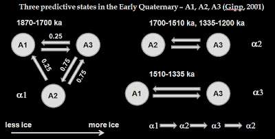
We observe three distinct interrelationships (epsilon machines) between our three predictive/successor states active during the Early Quaternary. The epsilon machines have been labelled α1, α2, α3 and each are active during different portions of the record (it may be that α2 and α3 simply represent limit cycles).
What does this tell us? From a computational standpoint, for α1--if the first predictive state was A1, then the next successor state is always A3. From A3, there is a 0.25 probability that A1 is the next successor, otherwise it is A2. From A2, there is a 0.75 probability that A3 is the next successor, otherwise it is A1. Given this information, one can use a stochastic process to generate a string of successor states that satisfy the criteria of the epsilon machine, but which would not necessarily be the exact sequence of observed states.
A climate model of this stage of the Quaternary could be readily tested against the observed model by testing to see whether there is a recognizable string of predictive/successor states in the output, and whether they satisfy (approximately) the observed probabilities (we should recognize that our observed probabilities may be relatively poor estimates of the actual probabilities). There are statistical tools for demonstrating the likelihood that the probabilities generated by the computer model are in agreement with the observed probabilities.

During the mid Quaternary, ice volume state A4 appears for the first time, and the epsilon machine (α4) shows increased complexity.

In the late Quaternary, the appearance of predictive state A5 ushers in a new, more complex epsilon machine I have called α5. The asymmetric sawtooth nature of glaciations in late Quaternary are reflected by the high probability of a rapid drop from A5 to A2 (p = 0.57), A3 (p = 0.14), or A1 via A6 (p = 0.14).
The five first-order epsilon machines we define through the Quaternary may be used as predictive/successor states and used to construct a second-order epsilon machine. There are not enough transitions to establish probabilities for transition from one second-order state to another, so our knowledge of this machine is lacking. At present it appears to be: α1, α2, α3, α2, α4, α5. It is a little more interesting than the second-order epsilon machine for the paleomonsoon proxy, but not completely satisfying. Nevertheless, it is still useful as a descriptor for the climate system, and can certainly be used to test computer models of climate.
Examples of testing models against the geologic record
Computer models of ice volume may be tested by determining the predictive or successor states from the model output, and comparing the resultant epsilon machines to the observed system. For a computer model to be considered successful, it should generate more than one first-order epsilon machine.
Let's try it.

Model 1: Parennin and Paillard (2003) model for Late Quaternary glacial cycles recognizes three metastable states: 1) an interglacial regime; 2) a mild glacial regime; and 3) a full glacial regime. The steps from one regime to another are driven by variable responses of the ice volume to northern hemisphere insolation modified by the extant ice volume. When in the mild glacial regime, ice volume does not drop suddenly in response to increasing insolation; nor does the system evolve back to the interglacial regime. Each transition from one state to another represents an irreversible change. Deglaciation only occurs from the full glacial regime in response to an increase in insolation.
The epsilon machine for this model output is summarized below.
. . . where I represents the interglacial regime, M represents mild glacial regime, and F represents the full glacial regime. In terms of the predictive/successor states used in the epsilon machine method, I corresponds to A2, M to A3, and F to A5.
The epsilon machine from the Paillard (2001) is simple, but no innovative behaviour is likely due to its tight definition. As there is only one first-order epsilon machine, there will clearly be no higher-order epsilon machines. Nor is it clear how to extend the model backward to the mid or early Quaternary.

A model constructed by Saltzman and Verbisky (1994) uses multiple feedbacks ('+' means positive feedback; '-' means negative) in order to generate a results which could be tested against a three-dimensional phase space defined by global ice volume, ocean temperature, and amospheric carbon dioxide. Interestingly, the resultant model successfully captured the multistability that characterizes the data; albeit one in which only two predictive/successor states are observed. The model was only run over a limited portion of the Late Quaternary, during an interval in which only states A2, A4, and A5 are observed.
If Kauffman's (1993) assertion that the number of metastable states (or Lyapunov-stable areas) in a complex system is a function of the square root of the number of parameters holds true, then the Saltzman-Verbitsky model has between about 1/2 and 1/9 of the number of parameters necessary to generate a model as complex in behaviour as the observed Late Quaternary ice volume proxy.
Nevertheless, the generation of multistability in this model represents a form of innovation (such multistability is not explicitly defined in the model), which places this model in my view above the Parennin and Paillard (2003) model--and indeed above virtually all other models of Late Quaternary climate encountered by this author.
Improperly nested epsilon machines in the geologic system
The observed first-order epsilon machines above (alpha-1 through alpha-5) can themselves be considered predictive or sucessor states (we shall call them second-order states to distinguish them from A1 through A5). The sequence of second-order states defines an epsilon machine of the second order. The second order epsilon machine, once completed, represents a third-order predictive or successor state, and given the number of such states, it may prove possible to define a third order epsilon machine.

Successively higher-ordered epsilon machines can be defined as long as there is data to support them. In theory there may be no limit to the order of machine that may be identified in geologic records; but in practice data are limited and we do not expect to easily rise above the second order epsilon machine.
For climate change, higher-order epsilon machines are expected to be related to higher-order cycles within earth history. Higher-order epsilon machines may relate to major tectonic events, and it may eventually prove possible to define epsilon machines of order W, related to Wilson cycles. Beyond that, would be a larger epsilon machine related to the formation (and eventual destruction) of Earth.
The heirarchy of computational processes necessarily reflects the heirarchy of geological processes. But these heirarchies are not perfectly nested. As related in the introduction, some of the results of Wilson-cycle dynamics feeds into the atmospheric circulation. As a consequence, the heirarchies are not nested, they are tangled. Such tangling of heirarchies is a requirement of innovative, complex behaviour (Hofstadter, 1979), and is no doubt the reason that such behaviour is a feature of geologic systems.
References
Casti, J., 1992. Reality Rules: Understanding the world through mathematics.
Crutchfield, J. P., 1994. The calculi of emergence: Computation, dynamics, and induction. Physica D 75: 11-54.
Gipp, M. R., 2001. Interpretation of climate dynamics from phase space portraits: Is the climate system strange or just different? Paleoceanography, 16, 335-351.
Gipp, M. R., in press. Imaging system change in reconstructed phase space: Evidence for multiple bifurcations in Quaternary paleoclimate. Paleoceanography.
Hofstadter, D., 1979. Godel, Escher, Bach: An Eternal Golden Braid.
Kauffman, S. (1993), The Origins of Order: Self-Organization and Selection in Evolution, Oxford Univ. Press, New York, 734 p.
Kukla, G., Z. S. An, J. L. Melice, J. Gavin, and J. L. Xiao, 1990. Magnetic susceptibility record of Chinese loess. Trans. R. Soc. Edinburgh Earth Sci., 81: 263-288.
Mañé, R.,1981. On the dimension of the compact invariant sets of certain non-linear maps, in Dynamical Systems and Turbulence, Warwick 1980, edited by D. Rand and L. S. Young, pp. 230-241, Springer-Verlag, New York.
Packard, N. H., J. P. Crutchfield, J. D. Farmer, and R. S. Shaw, 1980. Geometry from a time series, Phys. Rev. Lett., 45, 712-716.
Paillard, D., 2001. Glacial cycles: Toward a new paradigm. Reviews of Geophysics, 3: 325-346.
Parrenin, F. and D. Paillard (2003), Amplitude and phase of glacial cycles from a conceptual model, Earth Planet. Sci. Lett., 214, 243-250.
Saltzman, B., and Verbitsky, M., 1994. Late Pleistocene climatic trajectory in the phase space of global ice, ocean state, and CO2: Observations and theory. Paleoceanography, 9: 767–779.
Shackleton, N. J., A. Berger, and W. R. Peltier, 1990. An alternative astronomical calibration of the Lower Pleistocene timescale based on ODP site 677, Trans. R. Soc. Edinburgh, Earth Sci., 81: 251-261.
No comments:
Post a Comment